Posted on: August 19, 2025 | Reading time: 14 minutes | Word count: 2834 words | Author: Dang Duong Minh Nhat
Hello everyone, welcome back! We now continue with episode 6 of this series. In this installment, we’ll dive into some of the more difficult (and interesting) topics: the Blum–Micali sequential construction and the hardness of predicting the next bit of a PRG.
To get the most out of this post, I highly recommend you first read episode 5 and the other articles in this series to build the right background.
Alright — let’s get started!
A Sequential Construction: The Blum-Micali Method
Okay, let’s start with a sequential construction method, invented by Blum and Micali, which uses a pseudorandom generator (PRG) with a small stretch to build a PRG that can stretch to an arbitrary length.
Suppose $G$ is a PRG defined on $(\mathcal{S}, \mathcal{R} \times \mathcal{S})$, where $\mathcal{S}$ and $\mathcal{R}$ are two finite sets. For any polynomially bounded value $n \ge 1$, we can construct a new PRG $G’$ defined on $(\mathcal{S}, \mathcal{R}^n \times \mathcal{S})$. For $s \in \mathcal{S}$, we define:
$$ \begin{aligned} G’(s) & := \\ & s_0 \leftarrow s\\ & \text{for } i \leftarrow 1 \text{ to } n \text{ do}\\ &\qquad (r_i,s_i) \leftarrow G(s_{i-1})\\ & \text{output } (r_1,\ldots,r_n,s_n). \end{aligned} $$
We call $G’$ the n-fold sequential composition of $G$.
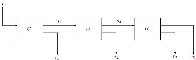 Figure 1: The sequential construction with $n = 3$
We will prove in Theorem 1 that if $G$ is a secure PRG, then $G’$ is also a secure PRG. A special case of this construction is as follows: suppose $G$ is a PRG defined on $(\left\lbrace 0,1\right\rbrace^\ell, \left\lbrace 0,1\right\rbrace^{t+\ell})$, where $\ell$ and $t$ are positive integers; that is, $G$ stretches an $\ell$-bit string into a $(t + \ell)$-bit string. We can view the output space of $G$ as $\left\lbrace 0,1\right\rbrace^t \times \left\lbrace 0,1\right\rbrace^\ell$, and by applying the above structure and interpreting the output as a bit string, we get a PRG $G’$ that stretches an $\ell$-bit string into an $(nt + \ell)$-bit string.
Theorem 1. If $G$ is a secure PRG, then its n-fold sequential composition $G’$ is also a secure PRG.
Specifically, for any PRG adversary $\mathcal{A}$ participating in the PRG Attack Game against $G’$, there exists a PRG adversary $\mathcal{B}$ participating in the PRG Attack Game against $G$, where $\mathcal{B}$ is simply a wrapper around $\mathcal{A}$, such that:
$$ \mathtt{PRG}\text{adv}[\mathcal{A}, G’] = n \cdot \mathtt{PRG}\text{adv}[\mathcal{B}, G]. $$
Proof. Let $\mathcal{A}$ be a PRG adversary participating in the PRG Attack Game against $G’$. We define a sequence of hybrid games, called Hybrid $0$, Hybrid $1$, …, Hybrid $n$. For $j = 0, 1, …, n$, Hybrid $j$ is defined as a game between $\mathcal{A}$ and a challenger as follows:
$$ \begin{aligned} & r_1 \xleftarrow{R} \mathcal{R}\\ & \vdots \\ & r_j \xleftarrow{R} \mathcal{R}\\ & s_j \xleftarrow{R} \mathcal{S}\\ & (r_{j+1},s_{j+1}) \leftarrow G(s_j)\\ & \vdots \\ & (r_n,s_n) \leftarrow G(s_{n-1})\\ & \text{send } (r_1,\ldots,r_n,s_n) \text{ to } \mathcal{A}. \end{aligned} $$
As usual, $\mathcal{A}$ will output $0$ or $1$ at the end of the game.
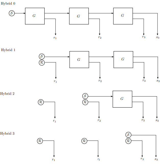 Figure 2: The challenger’s computation in the hybrid games with $n = 3$. Circles denote elements randomly generated from the set $\mathcal{S}$ or $\mathcal{R}$, as labeled.
Let $p_j$ be the probability that $\mathcal{A}$ outputs $1$ in Hybrid $j$. Note that $p_0$ is the probability that $\mathcal{A}$ outputs $1$ in Experiment 0 and $p_n$ is the probability that $\mathcal{A}$ outputs $1$ in Experiment 1 of the PRG Attack Game. Therefore, we have:
$$ \mathtt{PRG}\text{adv}[\mathcal{A}, G’] = |p_n - p_0| \quad \tag{1} $$
We next define a PRG adversary $\mathcal{B}$ participating in the PRG Attack Game against $G$, which operates as follows:
- Upon receiving $(r, s) \in \mathcal{R} \times \mathcal{S}$ from its challenger, $\mathcal{B}$ acts as a challenger for $\mathcal{A}$ as follows:
$$ \begin{aligned} & \omega \xleftarrow{R} \left\lbrace 1,\ldots,n\right\rbrace \\ & r_1 \xleftarrow{R} \mathcal{R}, \ldots , r_{\omega-1} \xleftarrow{R} \mathcal{R} \\ & (r_{\omega}, s_{\omega}) \leftarrow (r,s) \\ & (r_{\omega+1}, s_{\omega+1}) \leftarrow G(s_{\omega}),\ldots, (r_{n}, s_{n}) \leftarrow G(s_{n-1}) \\ & \text{send } (r_1,\ldots,r_n,s_n) \text{ to } \mathcal{A}. \end{aligned} $$
- Finally, $\mathcal{B}$ outputs whatever $A$ outputs.
Let $W_0$ be the event that $B$ outputs 1 in Experiment 0, and $W_1$ be the event that $B$ outputs 1 in Experiment 1 of the PRG Attack Game.
The key observation is:
For each $j = 1, …, n$, conditioning on $ω = j$ makes Experiment 0 for $\mathcal{B}$ equivalent to Hybrid $j-1$, and Experiment 1 for $\mathcal{B}$ equivalent to Hybrid $j$.
Therefore:
$$ \Pr[W_0 \mid ω = j] = p_{j-1} \quad \text{and} \quad \Pr[W_1 \mid ω = j] = p_j $$
The rest of the proof is a simple calculation, identical to the final part of the proof of Theorem 1 in the Cryptography 5 post. ✷
One criterion for evaluating a PRG is its expansion rate: a PRG that stretches an $n$-bit seed into an $m$-bit output has an expansion rate of $m/n$; more generally, if the seed space is $\mathcal{S}$ and the output space is $\mathcal{R}$, the expansion rate is defined as $\log |\mathcal{R}| / \log |\mathcal{S}|$. The sequential construction achieves a better expansion rate than a parallel construction. However, it has the disadvantage of not being parallelizable.
The Next-Bit Test
Suppose $G$ is a PRG defined on $(\left\lbrace 0,1\right\rbrace^{\ell},\left\lbrace 0,1\right\rbrace^{L})$, meaning it expands an $\ell$-bit string into an $L$-bit string. There are many ways an adversary could distinguish the pseudorandom output of $G$ from a truly random bit string. Indeed, suppose an efficient adversary could compute, for instance, the last bit of $G$’s output, given the first $L - 1$ bits. The existence of such an adversary would render $G$ insecure, because given the first $L - 1$ bits of a truly random $L$-bit string, the chance of guessing the last bit correctly should be just $50$–$50$.
We will formally define the notion of unpredictability for a PRG; in essence, this means that: for an adversary-chosen index $i$, given the first $i$ bits of $G$’s output, it is hard to predict the next bit (i.e., the $(i+1)$-th bit) with a probability significantly better than $1/2$. We will then prove that unpredictability and security are equivalent concepts. That security $\Rightarrow$ unpredictability is quite clear: if one can efficiently predict the next bit of a pseudorandom sequence, this immediately provides an effective statistical test. However, proving the reverse direction (unpredictability $\Rightarrow$ security) is much more interesting (and more difficult): this result states that if any efficient statistical test exists, then an efficient method for predicting the next bit in the pseudorandom sequence must also exist.
The Attack Game (PRG Unpredictability). For a PRG $G$ (defined on $(\mathcal{S}, \left\lbrace 0,1\right\rbrace^L)$) and an adversary $\mathcal{A}$, the attack game proceeds as follows:
The adversary sends an index $i$, with $0 \le i \le L-1$, to the challenger.
The challenger generates:
$$ s \xleftarrow{R} \mathcal{S},\quad r \leftarrow G(s), $$
and sends $r[0 \dots i-1]$ to the adversary.
The adversary outputs a bit $g \in \left\lbrace 0,1\right\rbrace$.
We say that $\mathcal{A}$ wins if $r[i] = g$, and we define the advantage of $A$:
$$ \mathtt{Pred}\text{adv}[\mathcal{A},G] := \bigl| \Pr[\mathcal{A} \text{ wins}] - 1/2 \bigr|. $$
$\square$
Definition (Unpredictable PRG). A PRG $G$ is called unpredictable if $\mathtt{Pred}\text{adv}[\mathcal{A},G]$ is negligible for all efficient adversaries $\mathcal{A}$.
We begin by proving that security $\Rightarrow$ unpredictability.
Theorem 2. Let $G$ be a PRG defined on $(\mathcal{S},\left\lbrace 0,1\right\rbrace^L)$. If $G$ is secure, then $G$ is unpredictable. More specifically, for every adversary $\mathcal{A}$ that breaks the unpredictability of $G$ in the Unpredictable PRG Game, there exists an adversary $\mathcal{B}$ that breaks the security of $G$ (in the PRG Game), such that $\mathcal{B}$ is just a simple wrapper around $\mathcal{A}$, and:
$$ \mathtt{Pred}\text{adv}[\mathcal{A},G] = \mathtt{PRG}\text{adv}[\mathcal{B},G]. $$
Proof. Let $\mathcal{A}$ be an adversary that breaks the unpredictability of $G$, and let $i$ be the index that $\mathcal{A}$ outputs. Assume $A$ wins the Unpredictable PRG Game with probability $1/2 + \varepsilon$, i.e., $\mathtt{Pred}\text{adv}[\mathcal{A},G] = |\varepsilon|$. We construct an adversary $\mathcal{B}$ that breaks the security of $G$ as follows:
Upon receiving $r \in \left\lbrace 0,1\right\rbrace^L$ from its challenger, $\mathcal{B}$ does the following:
- It gives $r[0 \dots i-1]$ to $\mathcal{A}$ and receives a guess $g \in \left\lbrace 0,1\right\rbrace$.
- If $r[i] = g$, $\mathcal{B}$ outputs $1$; otherwise, it outputs $0$.
Let $W_b$ be the event that $\mathcal{B}$ outputs $1$ in Experiment $b$ of the PRG Game ($b \in \left\lbrace 0,1\right\rbrace$).
In Experiment 0: $r$ is a pseudorandom output, so
$$ \Pr[W_0] = 1/2 + \varepsilon. $$
In Experiment 1: $r$ is a truly random string, but $r[i]$ and $g$ are independent, so
$$ \Pr[W_1] = 1/2. $$
Therefore:
$$ \mathtt{PRG}\text{adv}[\mathcal{B},G] = |\Pr[W_1] - \Pr[W_0]| = |\varepsilon| = \mathtt{Pred}\text{adv}[\mathcal{A},G]. \quad \square $$
The more interesting (and difficult) task is to prove the converse: unpredictability $\Rightarrow$ security. Before diving into the details of the proof, let’s sketch the high-level ideas:
First, we use a hybrid argument, which allows us to argue that if $\mathcal{A}$ can efficiently distinguish an $L$-bit pseudorandom string from an $L$-bit random string, then we can construct an efficient adversary $\mathcal{B}$ that can distinguish
$$ x_1 \cdots x_j x_{j+1} \quad\text{from}\quad x_1 \cdots x_j r, $$
where $j$ is a randomly chosen index, $x_1, \ldots, x_L$ are the pseudorandom outputs, and $r$ is a random bit. Thus, the adversary $\mathcal{B}$ can distinguish the pseudorandom bit $x_{j+1}$ from the random bit $r$, given the prefix string $x_1, \ldots, x_j$.
The final goal is to turn this distinguishing advantage into a predicting advantage. The rough idea is as follows: Given $x_1, \ldots, x_j$, we feed the adversary $\mathcal{B}$ the string $x_1, \ldots, x_j r$ where $r$ is randomly chosen.
- If $\mathcal{B}$ outputs $1$, we guess $x_{j+1} = r$;
- If $\mathcal{B}$ outputs $0$, we guess $x_{j+1} = \overline{r}$.
The fact that this prediction strategy works is due to the following general result, which we call the distinguisher/predictor lemma. The general setup is as follows:
$\mathbf{X}$ is a random variable, corresponding to the “side information” $x_1,\ldots,x_j$ above, as well as all the random coins used by the adversary $\mathcal{B}$;
$\mathbf{B}$ is a $0/1$-valued random variable, corresponding to $x_{j+1}$, which may depend on $\mathbf{X}$;
$\mathbf{R}$ is a $0/1$-valued random variable, corresponding to $r$ above, which is independent of $(\mathbf{X},\mathbf{B})$;
$d$ is a function, corresponding to $\mathcal{B}$’s strategy, such that $\mathcal{B}$’s distinguishing advantage is $|\varepsilon|$, where
$$ \varepsilon = \Pr[d(\mathbf{X},\mathbf{B}) = 1] - \Pr[d(\mathbf{X},\mathbf{R}) = 1]. $$
The lemma states that if we define the predictor variable $\mathbf{B}’$ according to the strategy above, specifically:
$$ \mathbf{B}’ = \begin{cases} \mathbf{R}, & \text{if } d(\mathbf{X},\mathbf{R}) = 1;\ \overline{\mathbf{R}}, & \text{if } d(\mathbf{X},\mathbf{R}) = 0, \end{cases} $$
then the probability that $\mathbf{B}’$ equals the true value $\mathbf{B}$ is precisely $1/2 + \varepsilon$. Here is the formal statement of the lemma:
Lemma (Distinguisher/predictor lemma). Let $\mathbf{X}$ be a random variable taking values in a set $S$, and let $\mathbf{B}, \mathbf{R}$ be $0/1$-valued random variables, where $\mathbf{R}$ is uniformly distributed on $\left\lbrace 0,1\right\rbrace$ and independent of $(\mathbf{X},\mathbf{B})$. Let $d : S \times \left\lbrace 0,1\right\rbrace \to \left\lbrace 0,1\right\rbrace$ be an arbitrary function, and set
$$ \varepsilon := \Pr[d(\mathbf{X},\mathbf{B}) = 1] - \Pr[d(\mathbf{X},\mathbf{R}) = 1]. $$
Define the random variable $\mathbf{B}’$ as follows:
$$ \mathbf{B}’ := \begin{cases} \mathbf{R}, & \text{if } d(\mathbf{X},\mathbf{R}) = 1,\\ \overline{\mathbf{R}}, & \text{if } d(\mathbf{X},\mathbf{R}) = 0. \end{cases} $$
Then
$$ \Pr[\mathbf{B}’ = \mathbf{B}] = \frac{1}{2} + \varepsilon. $$
Proof. We compute $\Pr[\mathbf{B}’ = \mathbf{B}]$ by conditioning on the two cases $\mathbf{B} = \mathbf{R}$ and $\mathbf{B} \ne \mathbf{R}$:
$$ \begin{aligned} \Pr[\mathbf{B}’ = \mathbf{B}] &= \Pr[\mathbf{B}’ = \mathbf{B} \mid \mathbf{B} = \mathbf{R}] \Pr[\mathbf{B}=\mathbf{R}] + \Pr[\mathbf{B}’ = \mathbf{B} \mid \mathbf{B} \ne \mathbf{R}] \Pr[\mathbf{B} \ne \mathbf{R}] \\ &= \Pr\bigl(d(\mathbf{X},\mathbf{R})=1 \big| \mathbf{B} = \mathbf{R}\bigr)\cdot\frac 12 \;+\; \Pr\bigl(d(\mathbf{X},\mathbf{R})=0 \big| \mathbf{B} \ne \mathbf{R}\bigr)\cdot\frac 12 \\ &= \frac 12\left(\Pr[d(\mathbf{X},\mathbf{R})=1 \mid \mathbf{B}=\mathbf{R}] + 1 - \Pr[d(\mathbf{X},\mathbf{R})=1 \mid \mathbf{B} \ne \mathbf{R}]\right) \\ &= \frac12 + \frac12(\alpha - \beta), \end{aligned} $$
where
$$ \alpha := \Pr[d(\mathbf{X},\mathbf{R})=1 \mid \mathbf{B} = \mathbf{R}], \qquad \beta := \Pr[d(\mathbf{X},\mathbf{R})=1 \mid \mathbf{B} \ne \mathbf{R}]. $$
Due to independence, we have
$$ \alpha = \Pr[d(\mathbf{X},\mathbf{R})=1 \mid \mathbf{B} = \mathbf{R}] = \Pr[d(\mathbf{X},\mathbf{B})=1 \mid \mathbf{B}=\mathbf{R}] = \Pr[d(\mathbf{X},\mathbf{B})=1]. $$
From this:
$$ \begin{aligned} \varepsilon &= \Pr[d(\mathbf{X},\mathbf{B})=1] - \Pr[d(\mathbf{X},\mathbf{R})=1] \\ &= \alpha - \left( \Pr[d(\mathbf{X},\mathbf{R})=1 \mid \mathbf{B}=\mathbf{R}]\Pr[\mathbf{B}=\mathbf{R}] + \Pr[d(\mathbf{X},\mathbf{R})=1 \mid \mathbf{B}\ne \mathbf{R}]\Pr[\mathbf{B}\ne \mathbf{R}] \right)\\ &= \alpha - \frac12(\alpha + \beta) = \frac12(\alpha - \beta), \end{aligned} $$
and substituting this into the formula above yields
$$ \Pr[\mathbf{B}’ = \mathbf{B}] = \frac12 + \varepsilon. $$
Theorem 3. Let $G$ be a PRG defined on $(S,\left\lbrace 0,1\right\rbrace^L)$. If $G$ is unpredictable, then $G$ is secure. Specifically, for every adversary $\mathcal{A}$ that breaks the security of $G$ (in the PRG Attack Game), there exists an adversary $\mathcal{B}$ that breaks the unpredictability of $G$ (in the Unpredictable PRG Game), where $\mathcal{B}$ is a simple wrapper around $\mathcal{A}$, such that
$$ \mathtt{PRG}\text{adv}[\mathcal{A}, G] = L \cdot \mathtt{Pred}\text{adv}[\mathcal{B}, G]. $$
Proof. Let $\mathcal{A}$ be an adversary against $G$ in the PRG Attack Game. Using $\mathcal{A}$, we construct a predictor $\mathcal{B}$ that attacks $G$ in the Unpredictable PRG Game as follows:
- Choose $\omega \in \left\lbrace 1,\ldots,L\right\rbrace$ uniformly at random.
- Send $L - \omega$ to its challenger and receive a prefix string $x \in \left\lbrace 0,1\right\rbrace^{L-\omega}$.
- Generate $\omega$ random bits $r_1,\ldots,r_\omega$, and send the $L$-bit string $x \Vert r_1\cdots r_\omega$ to $\mathcal{A}$.
- If $\mathcal{A}$ outputs $1$, then output $r_1$; otherwise, output $\overline{r_1}$.
To analyze $\mathcal{B}$, we consider $L+1$ hybrid games, called Hybrid 0, Hybrid 1, …, Hybrid $L$. For $j = 0,\ldots,L$, Hybrid $j$ is defined as a game between $\mathcal{A}$ and a challenger who creates a bit string $r$ consisting of:
- $L - j$ pseudorandom bits, followed by
- $j$ truly random bits.
That is, the challenger chooses $s \in S$ and $t \in \left\lbrace 0,1\right\rbrace^j$ uniformly at random and sends $\mathcal{A}$ the string
$$ r := G(s)[0..L-j-1] \Vert t. $$
As usual, $\mathcal{A}$ outputs $0$ or $1$ at the end of the game, and we denote by $p_j$ the probability that $\mathcal{A}$ outputs $1$ in Hybrid $j$. Note that $p_0$ is the probability that $\mathcal{A}$ outputs $1$ in Experiment 0 of the PRG Attack Game, while $p_L$ is the probability that $\mathcal{A}$ outputs $1$ in Experiment 1.
Let $W$ be the event that $\mathcal{B}$ wins the Unpredictable PRG Game (i.e., it correctly predicts the next bit). Then
$$ \begin{aligned} \Pr[W] &= \sum_{j=1}^{L} \Pr[W \mid \omega = j] \cdot \Pr[\omega = j] \\ &= \frac{1}{L} \sum_{j=1}^{L} \Pr[W \mid \omega = j] \\ &= \frac{1}{L} \sum_{j=1}^{L} \left( \frac12 + p_{j-1} - p_j \right)\quad\text{(by the Distinguisher/predictor lemma)} \\ &= \frac12 + \frac{1}{L}(p_0 - p_L), \end{aligned} $$
To explain the transformation above, we analyze the predictor adversary $\mathcal{B}$ by considering the Hybrid $j$ games. By the definition above:
$$ r := G(s)[0..L-j-1] \Vert t, $$
so we have:
Game Bits $1 \ldots L-j-1$ Bits $L-j \ldots L$ Hybrid $(j-1)$ Pseudorandom bit $x_{L-j}$ (pseudorandom), then $(j−1)$ random bits Hybrid $j$ Pseudorandom $j$ random bits Thus, the two Hybrids differ exactly at bit position $L-j$:
- In Hybrid $(j-1)$: it’s the true bit $x_{L-j}$ generated by the PRG.
- In Hybrid $j$: it’s a random bit $r$.
In adversary $\mathcal{B}$’s algorithm:
- The part $G(s)[0..L-j-1]$ serves as the side information $\mathbf{X}$ (known beforehand).
- $\mathcal{B}$ shows $\mathcal{A}$ the prefix $\mathbf{X}$ concatenated with a bit $b$ at position $L-j$.
- The bit $b$ is $x_{L-j}$ (if simulating Hybrid $(j-1)$) or a random $r$ (if simulating Hybrid $j$).
- $\mathcal{A}$ outputs $d(\mathbf{X},b)\in \left\lbrace 0,1\right\rbrace$.
- $\mathcal{B}$ then uses this output to predict the true bit $x_{L-j}$.
Distinguisher/predictor Lemma In our Proof $\mathbf{X}$ $G(s)[0..L-j-1]$ $\mathbf{B}$ The true bit $x_{L-j}$ $\mathbf{R}$ The random bit $r$ $d(\mathbf{X},\cdot)$ The output of $\mathcal{A}$ The Distinguisher/predictor lemma states that if the predictor uses the rule: If $d(\mathbf{X},\mathbf{R})=1$ → guess $\mathbf{B} = \mathbf{R}$, If $d(\mathbf{X},\mathbf{R})=0$ → guess $\mathbf{B} = \overline{\mathbf{R}}$ then
$$ \Pr[W\mid \omega=j] =\frac12 + \left(\Pr[d(\mathbf{X},\mathbf{B})=1] - \Pr[d(\mathbf{X},\mathbf{R})=1]\right). $$
Where:
- $\Pr[d(\mathbf{X},\mathbf{B})=1] = p_{j-1}$ (the probability $\mathcal{A}$ outputs $1$ in Hybrid $(j-1)$),
- $\Pr[d(\mathbf{X},\mathbf{R})=1] = p_j$ (the probability $\mathcal{A}$ outputs $1$ in Hybrid $j$).
Therefore:
$$ \Pr[W\mid \omega=j] = \frac12 + (p_{j-1} - p_j). $$
and it follows that
$$ \mathtt{Pred}\text{adv}[\mathcal{B}, G] = \left|\Pr[W] - \frac12\right| = \frac{1}{L} \cdot |p_0 - p_L| = \frac{1}{L} \cdot \mathtt{PRG}\text{adv}[\mathcal{A}, G]. $$
This implies
$$ \mathtt{PRG}\text{adv}[\mathcal{A}, G] = L \cdot \mathtt{Pred}\text{adv}[\mathcal{B}, G], $$
which proves the theorem. $\square$
In this blog, we have taken a deep dive into two foundational aspects of pseudorandom generators. We have seen how the Blum-Micali sequential construction offers an elegant method to amplify the length of a pseudorandom sequence while preserving its security.
Most importantly, we have proven the tight equivalence between security (statistical indistinguishability) and unpredictability (the hardness of guessing the next bit). This result is not just theoretically beautiful but also has immense practical significance: it simplifies the task of proving PRGs secure. Instead of confronting an infinite number of potential statistical tests, we only need to prove that predicting the next bit is computationally infeasible.
With a secure PRG in hand, we now possess one of the most fundamental building blocks of modern cryptography. In future articles, we will see how these blocks are used to construct more complex cryptographic systems, such as stream ciphers.
References
- Dan Boneh and Victor Shoup. A Graduate Course in Applied Cryptography. Retrieved from https://toc.cryptobook.us/
Connect with Me
Connect with me on Facebook, LinkedIn, via email at dangduongminhnhat2003@gmail.com, GitHub, or by phone at +84 829 258 815.