Posted on: November 5, 2025 | Reading time: 13 minutes | Word count: 2716 words | Author: Dang Duong Minh Nhat
Hello everyone! It’s been a while since my last post. In this eighth post, I’ll introduce the fundamentals of Lattices and the LLL algorithm. For a better understanding, please check out Part 7 and other posts in this cryptography series. Alright, let’s get started!
Lattices
Basic Definitions
Definition 1 (Lattice). An $n$-dimensional lattice $\mathcal{L}$ is a discrete subgroup (under addition) of $\mathbb{R}^n$.
A lattice can be described by a basis $\mathbf{B}$ containing linearly independent basis vectors $\left\lbrace \mathbf{b}_1, \ldots, \mathbf{b}_m\right\rbrace$ with $\mathbf{b}_i \in \mathbb{R}^n$. The number of vectors in the basis, $m$, is called the rank of the lattice. We primarily focus on full-rank lattices, which have the same rank and dimension, i.e., $m = n$.
The lattice can be seen as the set of all integer linear combinations of the basis vectors:
$$ \mathcal{L} = \mathcal{L}(\mathbf{B}) = \left\lbrace \sum_{i=1}^m a_i \mathbf{b}_i \Big| a_i \in \mathbb{Z} \right\rbrace $$
The figure below depicts a two-dimensional lattice. Note that any non-trivial lattice consists of infinitely many elements (called lattice points), but it is generated by linear combinations of the basis vectors.
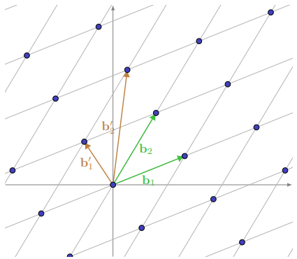
With this intuition, we see that a lattice basis is not unique. The figure above shows two different bases generating the same lattice.
In fact, every non-trivial lattice has infinitely many bases. However, although a lattice can be represented by many different bases, there exist special “good” bases, ideal for solving certain computational problems.
The next section defines some properties of lattices, helping us formalize the concept of a “good” basis and, ultimately, how to find one.
Properties, Invariants, and Characterizations
Two bases are bases for the same lattice if they generate exactly all points in the lattice.
But when a basis can take many different forms, how can we efficiently determine if two bases generate the same lattice? To answer this, we define some properties of lattice bases, as well as lattice invariants: quantities associated with the lattice that do not change depending on the basis.
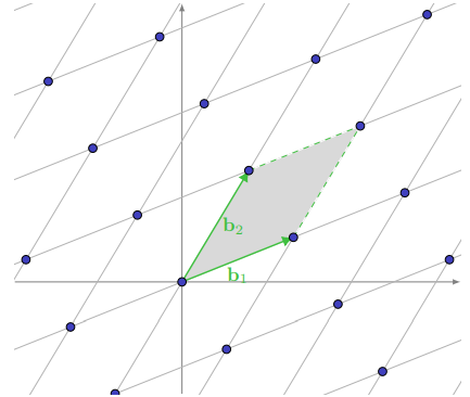
Definition 2 (Fundamental Parallelepiped). Given $\mathbf{B} = \left\lbrace \mathbf{b}_1, \ldots, \mathbf{b}_m\right\rbrace$ as a basis. The Fundamental Parallelepiped of $\mathbf{B}$ is defined as:
$$ \mathcal{P}(\mathbf{B}) = \left\lbrace \sum_{i=1}^m a_i \mathbf{b}_i \Big| a_i \in [0,1) \right\rbrace $$
The figure below shows a lattice and a basis, with the fundamental parallelepiped of the basis highlighted. Note that this region is half-open, and does not include the three non-zero lattice points (due to $a_i \in [0, 1)$).
In fact, one way to geometrically characterize a lattice basis is to observe whether its fundamental parallelepiped contains a non-zero lattice point. A basis $\mathbf{B}$ is a basis for a lattice $\mathcal{L}$ if and only if:
$$ \mathcal{P}(\mathbf{B}) \cap \mathcal{L} = \left\lbrace 0\right\rbrace $$
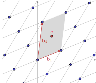
The vectors $\left\lbrace \mathbf{b}_1, \mathbf{b}_2\right\rbrace$ in the figure below do not form a basis because their fundamental parallelepiped contains a non-zero lattice point.
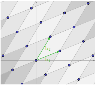
Conversely, if the fundamental parallelepiped contains only the zero vector, we can visualize it tiling the entirety of $\mathbb{R}^n$, with each tile containing exactly one lattice point, as in the figure below.
Clearly, different choices of basis will produce different fundamental parallelepipeds, even if both bases represent the same lattice. However, there is one invariant quantity: the volume of each fundamental parallelepiped, called the determinant of the lattice.
Definition 3 (Determinant). Let $\mathbf{B}$ be a basis for a full-rank lattice $\mathcal{L} = \mathcal{L}(\mathbf{B})$. The determinant of $\mathcal{L}$, denoted $\det(\mathcal{L})$, is the $n$-dimensional volume of $\mathcal{P}(\mathbf{B})$. We have:
$$ \det(\mathcal{L}) = \text{vol}(\mathcal{P}(\mathbf{B})) = |\det(\mathbf{B})| $$
It is not immediately obvious why the determinant is a lattice invariant. To prove this, we consider the algebraic characterization of lattice bases.
Suppose we have two bases $\mathbf{B} = \left\lbrace \mathbf{b}_1, \ldots, \mathbf{b}_n\right\rbrace$ and $\mathbf{B}’ = \left\lbrace \mathbf{b}’_1, \ldots, \mathbf{b}’_n\right\rbrace$ for a full-rank lattice $\mathcal{L}$.
Each vector $\mathbf{b}’_i$ is in the lattice, so it can be uniquely written as an integer linear combination of $\mathbf{b}_1, \ldots, \mathbf{b}_n$:
$$ \mathbf{b}’_1 = a_{11} \mathbf{b}_1 + \cdots + a_{1n} \mathbf{b}_n $$
$$ \vdots $$
$$ \mathbf{b}’_n = a_{n1} \mathbf{b}_1 + \cdots + a_{nn} \mathbf{b}_n $$
We can write the matrix equation $\mathbf{B}’ = \mathbf{A} \mathbf{B}$, where $\mathbf{A}$ is an integer matrix. Similarly, the $\mathbf{b}_i$ vectors can also be uniquely written as integer linear combinations of $\mathbf{b}’_i$. Specifically:
$$ \mathbf{B} = \mathbf{A}^{-1} \mathbf{B}' $$
Since $\mathbf{A}^{-1}$ must also be an integer matrix, we have:
$$ \det(\mathbf{A} \mathbf{A}^{-1}) = \det(\mathbf{A}) \det(\mathbf{A}^{-1}) = \det(\mathbf{I}) = 1 $$
where $\det(\mathbf{A})$ and $\det(\mathbf{A}^{-1})$ are both integers. Thus, $|\det(\mathbf{A})| = 1$.
Conversely, suppose there exists an integer matrix $\mathbf{A}$ with $|\det(\mathbf{A})| = 1$ such that $\mathbf{B} = \mathbf{A} \mathbf{B}’$. In this case, it is obvious that each vector in $\mathbf{B}$ can be written as an integer linear combination of the vectors in $\mathbf{B}’$, so $\mathcal{L}(\mathbf{B}) \subseteq \mathcal{L}(\mathbf{B}’)$. We also have $\mathbf{B}’ = \mathbf{A}^{-1} \mathbf{B}$, so by the same logic, we have $\mathcal{L}(\mathbf{B}’) \subseteq \mathcal{L}(\mathbf{B})$. Therefore, $\mathcal{L}(\mathbf{B}) = \mathcal{L}(\mathbf{B}’)$.
This leads to the following theorem, which will play an important role in the following sections.
Theorem 4. Let $\mathbf{B}$ and $\mathbf{B}’$ be bases. Then:
$$ \mathcal{L}(\mathbf{B}) = \mathcal{L}(\mathbf{B}’) \iff \mathbf{B} = \mathbf{U} \mathbf{B}' $$
where $\mathbf{U}$ is an integer matrix with $|\det(\mathbf{U})| = 1$.
From this theorem, we immediately see why the lattice determinant is an invariant. If $\mathbf{B}$ and $\mathbf{B}’$ are bases for the same lattice $\mathcal{L}$, then $\mathbf{B} = \mathbf{U} \mathbf{B}’$, so:
$$ \det(\mathbf{B}) = \det(\mathbf{U} \mathbf{B}’) = \det(\mathbf{U})\det(\mathbf{B}’) = \pm \det(\mathbf{B}’) $$
Thus, $|\det(\mathbf{B})| = |\det(\mathbf{B}’)|$.
The determinant is a useful property for analyzing algorithms and later geometric bounds.
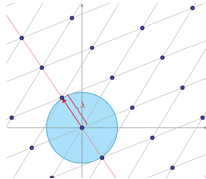
Another important lattice invariant is the successive minima. The first successive minimum, often denoted $\lambda(\mathcal{L})$ or simply $\lambda$, is the length of the shortest non-zero vector in the lattice.
In general, a rank $n$ lattice has $n$ successive minima, defined as follows:
Definition 5 (Successive Minima). Let $\mathcal{L}$ be a lattice of rank $n$. For $i \in \left\lbrace 1, \ldots, n\right\rbrace$, the $i$-th successive minimum of $\mathcal{L}$, denoted $\lambda_i(\mathcal{L})$, is the smallest radius $r$ such that $\mathcal{L}$ contains $i$ linearly independent vectors of length no more than $r$.
Geometrically, $\lambda_i(L)$ is the radius of the smallest closed ball around the origin containing $i$ linearly independent vectors. The figure below illustrates the first successive minimum of a lattice.
Interestingly, no efficient algorithm is known to compute the successive minima exactly. However, there is an upper bound given by Minkowski.
Theorem 6 (Minkowski’s First Theorem). Let $\mathcal{L}$ be a full-rank $n$-dimensional lattice. Then:
$$ \lambda_1(\mathcal{L}) \leq \sqrt{n} \cdot |\det(\mathcal{L})|^{1/n} $$
The first successive minimum is particularly important, as it provides a benchmark for evaluating the lengths of vectors in the lattice.
Problems on Lattices
We now define some important computational problems on lattices.
Definition 7 (Shortest Vector Problem – SVP). Given a basis $\mathbf{B}$ of a lattice $\mathcal{L} = \mathcal{L}(\mathbf{B})$, find a non-zero lattice vector $\mathbf{v}$ such that:
$$ \lVert \mathbf{v} \rVert = \lambda_1(L) $$
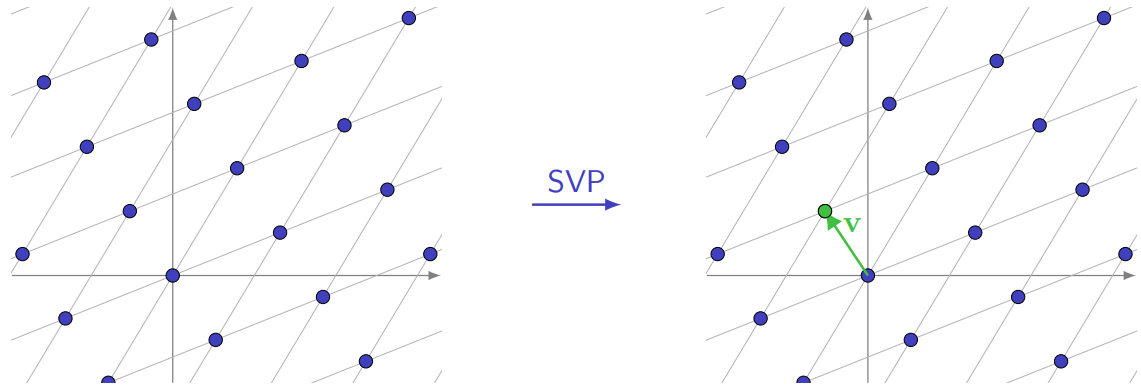 Figure: The Shortest Vector Problem.
Definition 8 (Closest Vector Problem – CVP). Given a basis $\mathbf{B}$ of a lattice $\mathcal{L} = \mathcal{L}(\mathbf{B})$ and a target vector $\mathbf{t}$ (not necessarily in $\mathcal{L}$), find a lattice vector $\mathbf{v}$ such that:
$$ \lVert \mathbf{v} - \mathbf{t} \rVert = \min_{\mathbf{w} \in \mathcal{L}} \lVert \mathbf{w} - \mathbf{t} \rVert $$
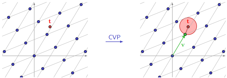 Figure: The Closest Vector Problem.
It is known that these problems are NP-Hard. However, we can define slightly “relaxed” versions of these problems, which do have efficient solutions for certain parameters. These versions will be more useful in cryptography.
Definition 9 (Approximate Shortest Vector Problem – $\textbf{SVP}_\gamma$). Given a basis $\mathbf{B}$ of a lattice $\mathcal{L} = \mathcal{L}(\mathbf{B})$ and an approximation factor $\gamma$, find a non-zero lattice vector $\mathbf{v}$ such that:
$$ \lVert \mathbf{v} \rVert \leq \gamma \cdot \lambda_1(\mathcal{L}) $$
Definition 10 (Approximate Closest Vector Problem – $\textbf{CVP}_\gamma$). Given a basis $\mathbf{B}$ of a lattice $\mathcal{L} = \mathcal{L}(\mathbf{B})$, a target vector $\mathbf{t}$, and an approximation factor $\gamma$, find a lattice vector $\mathbf{v}$ such that:
$$ \lVert \mathbf{v} - \mathbf{t} \rVert \leq \gamma \cdot \min_{\mathbf{w} \in \mathcal{L}} \lVert \mathbf{w} - \mathbf{t}\rVert $$
To solve these computational problems, we use lattice reduction. The idea is that we can transform any given lattice basis into a “better” basis, one that contains shorter and more orthogonal vectors.
In the next section, we will describe the LLL algorithm, a lattice reduction algorithm that provides a polynomial-time solution to these problems, with an approximation factor that is exponential in the dimension of the lattice.
Lattice Reduction
The goal of lattice reduction is to take an arbitrary lattice basis and transform it into another basis for the same lattice, where the vectors are shorter and more nearly orthogonal. Since we are looking for short vectors, this process itself can give us a solution to the approximate shortest vector problem.
Recall from Theorem 4 that two bases $\mathbf{B}$ and $\mathbf{B}’$ represent the same lattice if and only if $\mathbf{B} = \mathbf{U}\mathbf{B}’$ for an integer matrix $\mathbf{U}$ with $|\det(\mathbf{U})| = 1$. This leads us to two useful transformations that can be performed on a lattice basis: vector swapping and vector addition.
- Multiplying the basis on the left by a matrix $T_{i,j}$ gives us a new basis where the $i$-th and $j$-th basis vectors are swapped.
- Multiplying the basis on the left by a matrix $L_{i,j}(k)$ gives us a new basis where $k$ times the $j$-th basis vector is added to the $i$-th basis vector.
Note that both of these matrices have a determinant of $\pm 1$. These two elementary transformations are the key components of the LLL algorithm.
$$ T_{i,j} = \begin{bmatrix} 1 & & & & & \\ & \ddots & & & & \\ & & 0 & 1 & & \\ & & 1 & 0 & & \\ & & & & \ddots & \\ & & & & & 1 \end{bmatrix} $$
$$ L_{i,j}(k) = \begin{bmatrix} 1 & & & & & \\ & \ddots & & & & \\ & & 1 & & & \\ & & k & 1 & & \\ & & & & \ddots & \\ & & & & & 1 \end{bmatrix} $$
The LLL Algorithm
We now describe the algorithm by Lenstra, Lenstra, and Lovász.
The first step of this iterative algorithm is to take the basis $\mathbf{B} = \left\lbrace \mathbf{b}_1, \dots, \mathbf{b}_n\right\rbrace$ and compute an orthogonal basis using the Gram–Schmidt orthogonalization process. This orthogonal basis is not a valid basis for the lattice, but it will help us reduce the lattice basis. We denote $\mathbf{x} \cdot \mathbf{y} \equiv \langle \mathbf{x}, \mathbf{y}\rangle$ as the inner product.
The Gram–Schmidt process gives us orthogonal vectors $\mathbf{b}_1^*, \dots, \mathbf{b}_n^*$ and coefficients $\mu_{i,j}$ defined as follows:
$$ \mathbf{b}_i^* = \begin{cases} \mathbf{b}_i, & i = 1 \\ \mathbf{b}_i - \sum_{j=1}^{i-1} \mu_{i,j} \mathbf{b}_j^*, & 1 < i \leq n \end{cases} $$
$$ \mu_{i,j} = \frac{\langle \mathbf{b}_i, \mathbf{b}_j^* \rangle}{\langle \mathbf{b}_j^*, \mathbf{b}_j^* \rangle} $$
With this tool, we have the concept of an LLL-reduced basis, which is our final goal.
Definition 11 ($\delta$-LLL-reduced). Let $\delta \in (1/4, 1)$. A basis $\mathbf{B} = \left\lbrace \mathbf{b}_1, \dots, \mathbf{b}_n\right\rbrace$ is called $\delta$-LLL-reduced if:
- $|\mu_{i,j}| \leq \tfrac{1}{2}$ for all $i > j$ (the size-reduced condition).
- $(\delta - \mu_{i+1,i}^2)\lVert \mathbf{b}_i^* \rVert^2 \leq \lVert \mathbf{b}_{i+1}^* \rVert^2$ for all $1 \leq i \leq n-1$ (the Lovász condition).
The first condition relates to the lengths of the basis vectors but is not sufficient to guarantee that all basis vectors are short. The second condition adds a more local requirement between consecutive Gram–Schmidt vectors, essentially stating that the second vector cannot be much shorter than the first.
Algorithm 1: The LLL Algorithm
- function LLL(Basic ${\mathbf{b}_1, \dots, \mathbf{b}_n}$, $\delta$)
- $\quad$ while true do
- $\quad \quad$ for $i = 2$ to $n$ do $\quad$ $\quad$ $\quad$ $\quad$ $\quad$ $\quad$ $\quad$ $\quad$ $\quad$ $\quad$ ▷ size-reduction
- $\quad$ $\quad$ $\quad$ for $j = i-1$ to $1$ do
- $\quad$ $\quad$ $\quad$ $\quad$ $\mathbf{b}_i^*, \mu_{i,j} \leftarrow$ Gram-Schmidt($\mathbf{b}_1, \dots, \mathbf{b}_n$)
- $\quad$ $\quad$ $\quad$ $\quad$ $\mathbf{b}_i \leftarrow \mathbf{b}_i - \lfloor \mu_{i,j} \rceil \mathbf{b}_j$
- $\quad$ $\quad$ if $\exists i$ sao cho $(\delta - \mu_{i+1,i}^2)\lVert \mathbf{b}_i^* \rVert^2 > \lVert \mathbf{b}_{i+1}^* \rVert^2$ $\quad$ $\quad$ ▷ Lovász condition
- $\quad$ $\quad$ $\quad$ Swap $\mathbf{b}_i$ và $\mathbf{b}_{i+1}$
- $\quad$ $\quad$ else
- $\quad$ $\quad$ $\quad$ return $\left\lbrace \mathbf{b}_1, \dots, \mathbf{b}_n\right\rbrace$
However, LLL does not always find the shortest vector. But we can prove that it always finds a vector within an exponential approximation factor (in the dimension) of the shortest vector.
Theorem 13. Let $\mathbf{B} = \left\lbrace \mathbf{b}_1, \ldots, \mathbf{b}_n\right\rbrace$ be a basis of a lattice and $\mathbf{B}^{\ast} = \left\lbrace \mathbf{b}^{\ast}_1, \ldots, \mathbf{b}^{\ast}_n\right\rbrace$ be its corresponding Gram–Schmidt orthogonalization. Then:
$$ \lambda_1(\mathcal{L}(\mathbf{B})) \geq \min_{i \in \left\lbrace 1, \ldots, n\right\rbrace} \lVert \mathbf{b}^{\ast}_i \rVert $$
Proof. Let $\mathbf{x} = (x_1, \ldots, x_n) \in \mathbb{Z}^n$ be a non-zero vector. We consider the lattice point $\mathbf{xB}$ and show that its length is bounded below by $\min_{i \in \left\lbrace 1, \ldots, n\right\rbrace} \lVert \mathbf{b}^{\ast}_i \rVert$.
Let $j$ be the largest index such that $x_j \neq 0$. Then:
$$ |\langle \mathbf{xB}, \mathbf{b}^{\ast}_j \rangle| = \Big|\Big\langle \sum_{i=1}^n x_i \mathbf{b}_i , \mathbf{b}^{\ast}_j \Big\rangle\Big| = \Big|\sum_{i=1}^n x_i \langle \mathbf{b}_i , \mathbf{b}^{\ast}_j \rangle \Big| \quad \text{(by linearity of inner product)} $$
Since $\mathbf{b}_i$ and $\mathbf{b}^{\ast}_j$ are orthogonal when $j > i$ and $x_i = 0$ when $i > j$, we have: (Note: This is translating the user’s text. The actual properties are that $\langle \mathbf{b}_i, \mathbf{b}^{\ast}_j \rangle = 0$ for $i < j$ and $x_i = 0$ for $i > j$, causing the sum to collapse to the $i=j$ term.)
$$ |\langle \mathbf{xB}, \mathbf{b}^{\ast}_j \rangle| = |x_j| \langle \mathbf{b}_j , \mathbf{b}^{\ast}_j \rangle = |x_j| \cdot \lVert \mathbf{b}^{\ast}_j \rVert^2 $$
From the Cauchy–Schwarz inequality, we have:
$$ |\langle \mathbf{xB}, \mathbf{b}^{\ast}_j \rangle|^2 \leq \langle \mathbf{xB}, \mathbf{xB} \rangle \cdot \langle \mathbf{b}^{\ast}_j, \mathbf{b}^{\ast}_j \rangle = \lVert \mathbf{xB} \rVert^2 \cdot \lVert \mathbf{b}^{\ast}_j \rVert^2 $$
It follows that:
$$ |x_j| \cdot \lVert \mathbf{b}^{\ast}_j \rVert^2 \leq \lVert \mathbf{xB} \rVert \cdot \lVert \mathbf{b}^{\ast}_j \rVert \Longrightarrow |x_j| \cdot \lVert \mathbf{b}^{\ast}_j \rVert \leq \lVert \mathbf{xB} \rVert $$
Since $x_j \neq 0$ and is an integer, we have $|x_j| \geq 1$, thus:
$$ \lVert \mathbf{b}^{\ast}_j \rVert \leq \lVert \mathbf{xB} \rVert $$
It follows that:
$$ \min_{i \in \left\lbrace 1, \ldots, n\right\rbrace} \lVert \mathbf{b}^{\ast}_i \rVert \leq \lVert \mathbf{xB} \rVert $$
Since $\mathbf{xB}$ can be any non-zero lattice point, we conclude that:
$$ \lambda_1(\mathcal{L}(\mathbf{B})) \geq \min_{i \in \left\lbrace 1, \ldots, n\right\rbrace} \lVert \mathbf{b}^{\ast}_i \rVert $$
Proposition 14. Let $\mathbf{B} = \left\lbrace \mathbf{b}_1, \ldots, \mathbf{b}_n\right\rbrace$ be a $\delta$-LLL-reduced basis. Then:
$$ \lVert \mathbf{b}_1 \rVert \leq \Bigg(\frac{2}{\sqrt{4\delta - 1}}\Bigg)^{n-1} \lambda_1 $$
Proof. From the Lovász condition, we have:
$$ (\delta - \mu_{i+1,i}^2)\lVert \mathbf{b}^{\ast}_i \rVert^2 \leq \lVert \mathbf{b}^{\ast}_{i+1} \rVert^2 $$
From the size-reduced condition, we have $|\mu_{i+1,i}| \leq \tfrac{1}{2}$. Therefore:
$$ \Big(\frac{4\delta - 1}{4}\Big)\lVert \mathbf{b}^{\ast}_i \rVert^2 \leq \lVert \mathbf{b}^{\ast}_{i+1} \rVert^2 $$
Combining the successive inequalities, we get:
$$ \lVert \mathbf{b}^{\ast}_1 \rVert^2 = \lVert \mathbf{b}_1 \rVert^2 \leq \Big(\frac{4}{4\delta - 1}\Big)^{i-1} \lVert \mathbf{b}^{\ast}_i \rVert^2 $$
which implies:
$$ \lVert \mathbf{b}_1 \rVert \leq \Big(\frac{2}{\sqrt{4\delta - 1}}\Big)^{i-1} \lVert \mathbf{b}^{\ast}_i \rVert $$
In particular, for $i = n$:
$$ \lVert \mathbf{b}_1 \rVert \leq \Big(\frac{2}{\sqrt{4\delta - 1}}\Big)^{n-1} \lVert \mathbf{b}^{\ast}_n \rVert $$
Proposition 15.
$$ \lVert \mathbf{b}_1 \rVert \leq \Big(\frac{2}{\sqrt{4\delta - 1}}\Big)^{n-1} \cdot \sqrt{n} \cdot |\det(\mathcal{L})|^{1/n} $$
This result is important because it gives us a rough estimate of the short vectors that LLL can find.
If we can model a specific problem where a solution exists as a short vector in some lattice, we can then solve it using lattice reduction, provided that the short vector falls within the exponential approximation factor of the shortest vector.
We have explored the fundamental concepts of lattices, from their geometric definition to their algebraic characterizations and core hard problems. The centerpiece of this blog is the LLL algorithm, a revolutionary tool for lattice basis reduction.
While LLL does not solve the Shortest Vector Problem (SVP) exactly, it provides a critical guarantee: in polynomial time, it can find a vector $\mathbf{b}_1$ whose length is only larger than the true shortest vector ($\lambda_1$) by an approximation factor (which is exponential in the dimension).
This balance—being inefficient enough to not break SVP completely, yet efficient enough to find “relatively short” vectors—makes LLL an incredibly powerful cryptanalytic tool. It serves as the foundation for both attacking weaker cryptosystems and as a benchmark for designing secure lattice-based cryptosystems, which are considered the future of cryptography in the post-quantum era.
References
- Joseph Surin and Shaanan Cohney. (2023). A Gentle Tutorial for Lattice-Based Cryptanalysis. Retrieved from https://eprint.iacr.org/2023/032.pdf
Connect with Me
Connect with me on Facebook, LinkedIn, via email at dangduongminhnhat2003@gmail.com, GitHub, or by phone at +84 829 258 815.