Posted on: August 14, 2024 | Reading time: 18 minutes | Word count: 3780 words | Author: Dang Duong Minh Nhat
In our previous blog, we delved into the fascinating world of Zero-Knowledge Proofs and their pivotal role in cryptography. Building on that foundation, this blog takes you on a journey through the essential concepts of polynomials, pairings, and commitment schemes—key tools that drive the magic behind secure cryptographic protocols. Whether you’re curious about how polynomials help smooth video transmission or intrigued by the mechanics of pairing-based cryptography, this guide will unravel the complex, making it accessible and engaging for all.
Table of Contents
- Table of Contents
- Polynomials
- Unlocking the Magic of Pairings: A Key to Modern Cryptography
- Commitment Schemes
- References
- Connect with Me
Polynomials
Understanding Polynomials in Cryptography: A Simple Guide
Polynomials are more than just mathematical expressions you encounter in school—they are powerful tools with wide-ranging applications, especially in the field of cryptography. But what exactly are polynomials, and why are they so crucial?
What Are Polynomials?
At their core, polynomials are expressions made up of variables like $x$ combined using basic operations: addition, subtraction, and multiplication. Each piece of the expression, known as a term, includes a variable (like $x$) and often a coefficient, which is just a number multiplying the variable.
For example, a simple polynomial might look like this: $$P(x) = a_nx^n + a_{n - 1}x^{n - 1} + \dots + a_2x^2 + a_1x + a_0$$
Here, each $a_i$ represents a coefficient, and the highest exponent of $x$ (in this case, $n$) gives us the degree of the polynomial. This degree is important because it tells us how complex the polynomial is.
Polynomials in Cryptography
In cryptography, polynomials aren’t just any mathematical expressions—they’re specifically defined over the integers, meaning both the coefficients and the values of $x$ are whole numbers. This makes sure that the results of these polynomials are also whole numbers.
One common way polynomials are used in cryptography is with modular arithmetic. This might sound complicated, but it’s just a fancy way of saying that we look at the remainder when a polynomial is divided by a number, called the modulus $m$.
So, if you see something like $P(x)$ mod $m$, it’s just a polynomial being worked with under these special rules. This approach is what we call working with polynomials over rings or finite fields, and it’s essential for many cryptographic systems.
Mastering the Art of Interpolation: Connecting the Dots in Cryptography
Interpolation might sound like a complex mathematical term, but it’s actually a fascinating process that plays a crucial role in connecting the dots—literally! Imagine you have a set of points on a graph, and you want to draw a smooth curve that passes through each one. Interpolation is the mathematical technique that makes this possible, and in cryptography, it’s a powerful tool for creating secure systems.
What is Interpolation?
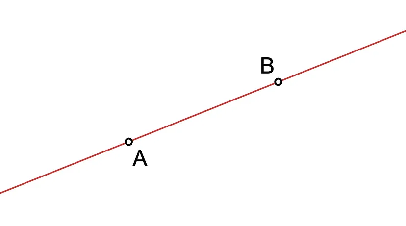
Interpolation is all about constructing a polynomial—a mathematical expression that involves variables and coefficients—that passes through a specific set of points. For instance, if you have two points on a graph, there’s only one straight line that connects them. This line can be described by a simple polynomial equation like this: $$P(x) = mx+n$$ where $m$ is the slope of the line and $n$ is where the line crosses the y-axis.
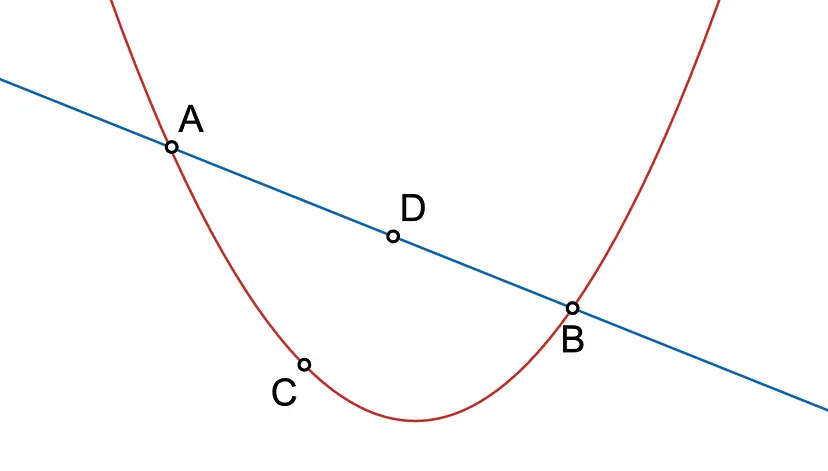
Now, what if you have three points? If the points are perfectly aligned (collinear), the same line could pass through them all. But if they’re not aligned, you’ll need a different approach. In this case, a unique curve, specifically a parabola (which is a degree-2 polynomial), will connect these three points.
The Power of Lagrange Polynomials
The concept of interpolation becomes even more interesting with Lagrange polynomials. When you have $m$ distinct points, there exists a unique polynomial of degree at most $m-1$ that passes through all of them. This polynomial is known as the Lagrange Polynomial.
For example, suppose you have three points represented as $(x_1, y_1), (x_2, y_2)$, and $(x_3, y_3)$. The Lagrange polynomial that connects these points can be written as: $$L(x) = ax^2 + bx+c$$ This polynomial is crafted to precisely pass through each of your specified points. The beauty of the Lagrange polynomial is that it’s not just a random curve—it’s the only curve of its kind that fits all the given points perfectly.
How Polynomials Help Keep Your Videos Smooth: The Magic of Erasure Coding
Have you ever sent a video through a messaging app and wondered how it arrives perfectly on the other end? It might seem like magic, but there’s actually some serious math behind the scenes making sure your video plays smoothly. One of the key techniques used to ensure that data arrives intact is called erasure coding—and it’s all about making sure nothing gets lost in transmission.
The Journey of Data: How Packet Loss Happens
When you send a video, the data isn’t sent as one big file. Instead, it’s broken down into smaller, manageable pieces called packets. Each packet is like a puzzle piece that, when put together, forms the complete video. But as these packets travel through the internet, some can get lost or damaged. This is where things get tricky.
Imagine you’re mailing a 10-piece puzzle, but when it arrives, 2 pieces are missing. Normally, you’d be stuck with an incomplete puzzle. Thankfully, technologies like Transmission Control Protocol (TCP) work hard to prevent this. If a packet doesn’t arrive, TCP asks for it again until the full puzzle (or video) is reassembled.
Beating Packet Loss with Redundancy
But there’s another clever trick to handle packet loss: redundancy. Redundancy means sending extra information so that even if some packets go missing, you can still put the puzzle together.
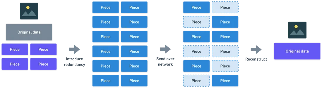
Let’s say you have a video divided into four chunks of data. Instead of just sending those four chunks, you might send six. That way, if two chunks are lost along the way, the remaining four are enough to recreate the entire video.
The Polynomial Puzzle: How Erasure Coding Works
Here’s where the magic of polynomials comes in. In erasure coding, the original data chunks are treated like coefficients in a polynomial—a special kind of mathematical equation.
For example, imagine each chunk of data is a number. We use these numbers as coefficients to create a polynomial, like this: $$P(x) = a_0 + a_1x + a_2x^2 + \dots + a_{m-1}x^{m-1}$$ where $m$ is the number of original data chunks.
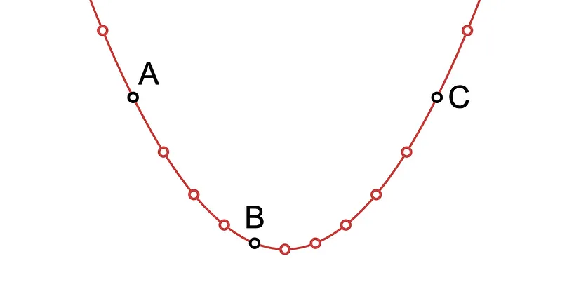
To send the data, we evaluate this polynomial at several different points (more than the number of chunks). Each result is sent as a packet over the network. The beauty of this method is that even if some of these packets are lost, the recipient can use the remaining ones to reconstruct the original polynomial using a technique called Lagrange interpolation. Once the polynomial is rebuilt, the original video data is fully recovered.
The Power of Direct Interpolation: Connecting the Dots with Polynomials
Interpolation is like connecting the dots in a drawing—except in mathematics, these “dots” are points on a graph, and the “lines” connecting them are curves described by polynomials. But how do we find the perfect curve that passes through all the points? This is where direct interpolation comes into play.
What Is Direct Interpolation?
Imagine you have a set of points on a graph, and you want to find a smooth curve that passes through each one. This curve is called an interpolating polynomial. The process of finding this polynomial is what we call interpolation.
The direct method of interpolation is straightforward. You start by setting up a system of linear equations based on your points, which you then solve to find the polynomial that fits. In other words, if you know where the dots are, you can calculate the exact curve that connects them. Using these points, you can write equations that describe how they relate to a polynomial like: $$L(x) - \sum_{j = 0}^k y_j l_j(x)$$ , where $$l_j(x)= \prod_{0 \leq m \leq k, m \neq j} \frac{x - x_m}{x_j - x_m} $$
The Challenge of Efficiency
While the direct method works perfectly well, it has a downside—it’s not the most efficient way to do interpolation, especially when you’re dealing with a large number of points. The reason for this is the method’s computational complexity, denoted as $O\left( n^2 \right)$, where $n$ is the number of points.
Think of it like this: if you’re trying to connect just a few dots, it’s no big deal. But if you have hundreds or thousands of points, the direct method can become slow and cumbersome, requiring a lot of calculations to get the job done.
Unlocking the Magic of Pairings: A Key to Modern Cryptography
In the world of cryptography, pairings are like a secret handshake between groups of numbers, enabling powerful and secure communication. But what exactly are pairings, and why are they so important? Let’s dive into this fascinating concept.
What Are Pairings?
At its core, a pairing is a special function that connects three groups of numbers, each with its own unique structure. These groups, denoted as $\mathbb{G}_1$, $\mathbb{G}_2$, and $\mathbb{G}_T$, have a prime number of elements, and pairings map elements from the first two groups ($\mathbb{G}_1$ and $\mathbb{G}_2$) to the third group ($\mathbb{G}_T$).
A pairing can be symmetric or asymmetric:
- Symmetric Pairing: $\mathbb{G}_1$ and $\mathbb{G}_2$ are the same group.
- Asymmetric Pairing: $\mathbb{G}_1$ and $\mathbb{G}_2$ are different groups.
But the real magic of pairings lies in their two main properties: bilinearity and non-degeneracy.
The Power of Bilinearity
Bilinearity is the property that makes pairings incredibly useful. In simple terms, it means that the pairing function maintains a linear relationship between the inputs. Imagine you’re multiplying two numbers, but you can switch the order of the operations without changing the result. This is what bilinearity allows you to do with more complex mathematical objects.
For example, if you have elements $u$ in $\mathbb{G}_1$ and $v$ in $\mathbb{G}_2$, and you apply the pairing function, you get the same result whether you combine the elements first or apply the pairing and then combine them. This flexibility is crucial in many cryptographic protocols, where it allows for sophisticated tricks that keep data secure.
Bilinearity requires that, for all $u \in \mathbb{G}_1$ , $v \in \mathbb{G}_2$ , and $a,b \in \mathbb{Z}_p$: $$e\left(u^a, v^b\right) = e(u, v)^{ab}$$
Why Non-Degeneracy Matters
The second key property, non-degeneracy, ensures that the pairing function is meaningful. Without this property, all the hard work of applying the pairing could be wasted, as it would collapse all inputs to a single, useless output. Non-degeneracy guarantees that the pairing function distinguishes between different inputs, making it a powerful tool for encryption and other cryptographic tasks.
Non-degeneracy requires that: $$e\left(g_1,g_2\right) \neq 1_{\mathbb{G}_T}$$
Pairings and Elliptic Curves: A Perfect Match
In practice, pairings often involve elliptic curves—geometric shapes that have become the backbone of modern cryptography. Elliptic curves are chosen because they are not only mathematically elegant but also computationally efficient. This efficiency makes them ideal for the complex calculations required in cryptographic protocols.
When using elliptic curves, pairings can be set up between two different groups or within the same group. In the latter case, a special mapping function transforms one group into the other, allowing the pairing to work within a single group—a technique known as self-pairing.
This means that all of the following are equivalent: $$e\left([a]G_1, [b]G_2\right) = e\left(G_1, [b]G_2\right)^a = e\left(G_1, G_2\right)^{ab} = e\left([b]G_1, [a]G_2\right)$$
Commitment Schemes
Unveiling the Power of Polynomial Commitments in Cryptography
When it comes to cryptography, concealing and revealing information is a delicate dance. We’ve all encountered the concept of a commitment scheme, where one party locks in a secret value and later reveals it to another party. But what if we could take this concept a step further—not just hiding a single secret, but an entire mathematical function? Enter the world of polynomial commitments, a fascinating and powerful tool in modern cryptography.
What Is a Polynomial Commitment?
Imagine you have a secret mathematical function, like a polynomial. Instead of revealing the entire function, you only want to share specific outputs, or evaluations, of this function at certain points. A polynomial commitment allows you to do just that. It lets you “commit” to the entire polynomial, locking it in securely, while giving you the flexibility to share only the parts of it that are necessary.
Here’s how it works: You create a commitment to the polynomial, which acts like a sealed envelope containing the full function. Then, when someone asks for the value of the polynomial at a specific point, you can provide that value along with a proof that confirms it’s accurate—all without revealing the full polynomial. This is like showing someone a snippet of your secret code while convincing them it’s part of a much larger, correct program.
The following diagram offers a simplified overview of this concept:
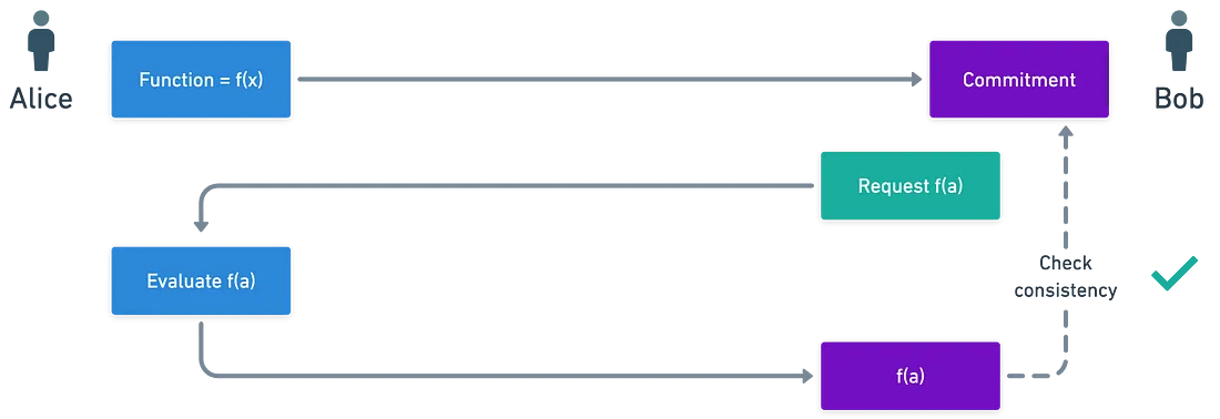
In this setup, the function $f$ remains secret and is never disclosed in its entirety. As hinted, the consistency check for this commitment will be facilitated by the use of pairings, which are vital for maintaining the integrity and security of the scheme.
Why Does This Matter?
You might wonder why such a complex mechanism is needed. The answer lies in the world of Zero-Knowledge Proofs (ZKPs) and threshold cryptography. In these advanced cryptographic protocols, proving the accuracy of information without revealing the underlying data is crucial. Polynomial commitments are key to ensuring that even when multiple parties are involved, the shared information remains accurate and secure.
For example, in verifiable secret sharing, which is a part of threshold cryptography, you don’t just want to share parts of a secret—you want to prove that the parts are correct. Polynomial commitments make this possible by allowing participants to verify the shared pieces of a secret without needing access to the entire secret.
Setting Up a Commitment Scheme: The Journey from Trust to Security
When diving into the world of cryptographic commitment schemes, it’s crucial to understand the foundational steps that make these protocols secure and reliable. Think of it as setting up a digital vault where secrets can be locked away safely, but with a catch—only certain people can verify what’s inside without opening it entirely. This journey begins with the initial setup and moves through to a trusted setup phase, both of which are vital to the integrity of the system.
Initial Setup
To begin, we need two groups of order n, which we will denote as $\mathbb{G}_1$ and $\mathbb{G}_3$. Additionally, a generator for $\mathbb{G}_1$, labeled as $G$, is required. These groups are generated to allow for the existence of a symmetric pairing (or self-pairing) in the form: $$e:\mathbb{G}_1 \times \mathbb{G}_2 \rightarrow \mathbb{G}_3$$ Given that we will be working with polynomials, we will use multiplicative notation to represent the elements of 𝔾1. This means that our group will take the form:
$\mathbb{G}_1 = $ { $G^s|s \in \mathbb{Z}_n$ }
A noteworthy point is that since $G$ will be input into a polynomial, and we frequently use elliptic curve groups in our examples, there is a minor complication. On an elliptic curve, points are typically multiplied by a scalar (i.e., $[s]G$) rather than exponentiated.
To resolve this, we can utilize an isomorphism into a multiplicative group, following similar reasoning to what is commonly used in cryptographic contexts. Therefore, $G^s$ will simply be interpreted as $[s]G$ in this setup.
Trusted Setup
The process requires what is known as a trusted setup. This means the system must be initialized with the calculation of certain public parameters, which are crucial for the verification phase.
We aim to commit to a polynomial of degree at most $d$. To achieve this, a trusted entity generates a random integer $\alpha$ and uses it to calculate the following set of public parameters: $$p=\left(H_0=G,H_1=G^\alpha,H_2=G^{\alpha ^2}, \dots, H_d=G^{\alpha ^d}\right) \in \mathbb{G}^{d + 1}$$ After generating these values, $\alpha$ must be discarded. Retaining knowledge of $\alpha$ could allow for the forging of false proofs, which is why the trustworthiness of the actor performing this action is essential. We will explore how false proofs could be generated later in the discussion.
Committing to the Polynomial
With the public parameters $p$ established, we can now proceed to create the actual commitment to a polynomial. The commitment itself will be represented by a single functional value, which we will denote using the tilde notation $\tilde{f} = G^{f(a)} \in \mathbb{G}$ to indicate that it is a commitment to a function. At first glance, it may seem that the secret value $\alpha$ is essential for computing the commitment. However, recall that $\alpha$ was discarded after the setup phase. This raises the question: how can we compute the commitment without access to $\alpha$?
The answer lies in the public parameters generated during the setup. Suppose we have a polynomial $f(x)$ of degree $d$ expressed as: $$f(x) = a_0 + a_1x + a_2x^2 + \dots + a_dx^d$$ We can utilize the public parameters to compute the following product: $$S = H_0^{a_0}.H_1^{a_1}.H_2^{a_2} \dots H_d^{a_d}$$ By simplifying the expression, we observe: $$S = G^{a_0}.G^{\alpha .a_1}.G^{\alpha ^2.a_2} \dots G^{\alpha ^d.a_d} = G^{a_0 + \alpha .a_1 + \alpha ^2.a_2 + \dots + \alpha ^d.a_d} = G^{f(\alpha)}$$ This expression represents the commitment to the polynomial $f(x)$, calculated without directly knowing $\alpha$. The prover computes this commitment value and sends it to the verifier. The verifier stores this value and uses it later to confirm the correctness of polynomial evaluations provided by the prover.
Evaluation
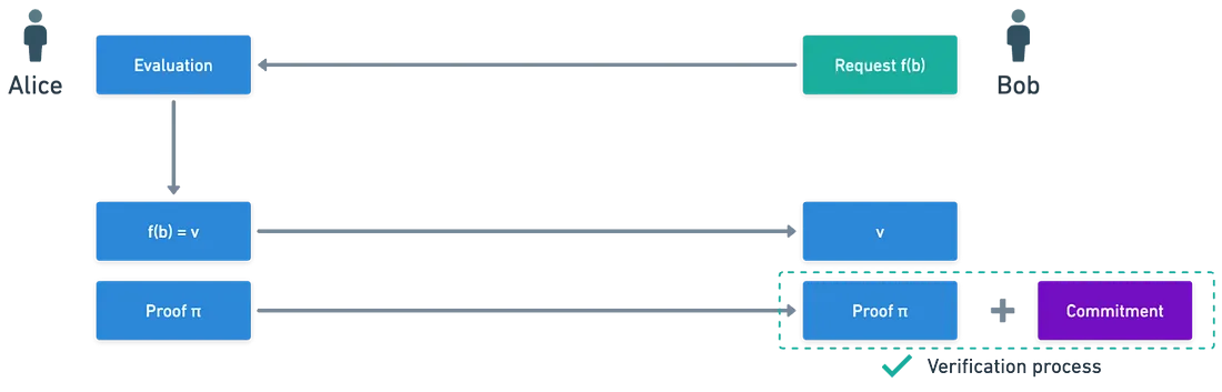
With the commitment established, the verifier can request evaluations of the secret polynomial. Specifically, the verifier may want to know the value of the polynomial $f(x)$ at a particular integer $b$. In this case, the verifier asks for $f(b)$. $$f(b) = a_0 + a_1b + a_2b^2 + \dots + a_db^d$$ The prover can compute this value and send it to the verifier. However, the verifier needs to ensure that the value provided is accurate and consistent with the original commitment, rather than a random or meaningless value.
To validate this, the prover must also generate a short proof that the verifier can use to confirm the correctness of the evaluation against the commitment they hold.
Proof Generation
To reiterate, the goal is to prove that $f(b)=v$. By rearranging the equation, it can also be expressed as: $$f(x)-v=(x-b).p(x)$$ This implies that $b$ is a root of the polynomial $\hat{g}(x)=f(x)-v$.
According to the factor theorem, the polynomial $f(x)-v$ can be perfectly divided by the polynomial $(x-b)$ without any remainder. The quotient $p(x)$ is the polynomial that satisfies the equation: $$f(x)-v=(x-b).p(x)$$ Next, a commitment to the polynomial $p(x)$ is calculated using the public parameters, just as it was done for $f(x)$. This commitment serves as the short proof needed by the verifier. The process can be visually updated as follows:
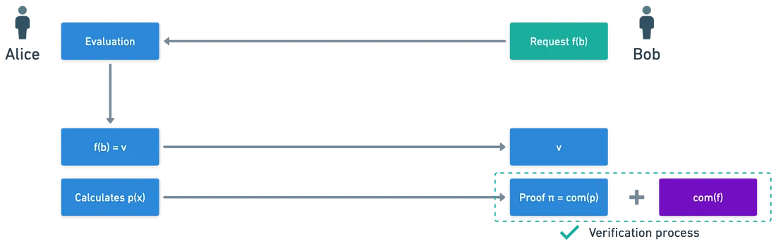
Upon receiving the polynomial evaluation v and the commitment to $p(x)$, the verifier can check the consistency of these values with the original commitment. This verification step ensures that the evaluation is accurate and trustworthy.
Verification
In simple terms, the verifier will accept the evaluation of the polynomial only if the following validation holds true: $$\tilde{p}^{(\alpha - b)} = \tilde{f}.G^{-v}$$ However, there is a challenge here: since α has been discarded, it remains unknown. We will discuss how to overcome this issue shortly. First, let’s ensure that this validation expression is meaningful.
Recall that the commitment for a polynomial $f$ is given by the value: $$\tilde{f} = G^{f(a)} \in \mathbb{G}$$ We have previously outlined how to calculate this commitment using the public parameters. Substituting this into the validation expression, we can rewrite it as: $$\left(G^{p(\alpha)}\right)^{(\alpha - b)} = G^{f(a)}.G^{-v}$$ Examining just the exponents, we see that: $$p(\alpha)(\alpha - b) = f(a) - v$$ If $p(x)$ was calculated and evaluated correctly, we know that the expressions $(α-b).p(α)$ and $f(α)-v$ should be equal. Therefore, the verification procedure is coherent.
This leads us to recognize why knowledge of $\alpha$ could allow for the creation of false proofs. For instance, I could send you an arbitrary number A instead of $f(\alpha)$ as the initial commitment. Without knowledge of $\alpha$ you would have no means to identify this as illegitimate. Subsequently, knowing $\alpha$, I could select any arbitrary value $v$ and falsely convince you that $f(b)=v$ by simply calculating and sending you the value of $P$: $$P = \frac{A-v}{\alpha - b}$$ This scenario highlights the importance of discarding α to prevent such fraudulent activities.
Pairing Mechanism
Here is where the concept of pairings becomes essential. The process works as follows, and we will verify its validity without requiring extensive motivation.
To introduce some terminology, we will refer to the commitment to $p(x)$, which is related to the value $b$, as a witness. We denote this witness by $w(b)$: $$w(b) = G^{p(\alpha)} = G^{\frac{f(\alpha) - f(b)}{\alpha - b}}$$ The objective is to verify that this witness is consistent with the commitment to $f$. For this purpose, we will evaluate our pairing and check the following condition: $$e\left(w(b), G^{\alpha}.G^{-b}\right).e(G, G)^{f(b)} = e\left(\tilde{f}, G\right)$$ The equality holds true only if $w(b)$ is calculated correctly, which can only occur if the prover indeed knows the secret polynomial.
Formally, we can establish the equality through the bilinearity property of the pairing:
$$ e\left(w(b), G^{\alpha}.G^{-b}\right).e(G, G)^{f(b)} = e\left(w(b), G^{\alpha - b}\right).e(G, G)^{f(b)} $$
$$= e(G, G)^{p(\alpha)(\alpha - b)}.e(G,G)^{f(b)} = e(G,G)^{p(\alpha)(\alpha -b) + f(b)}$$ $$= e(G, G)^{f(\alpha)} = e\left(G^{f(\alpha)}, G\right) = e\left(\tilde{f}, G\right)$$ This pairing mechanism provides a secure means for verification, ensuring that the evaluations are consistent without requiring knowledge of $\alpha$.
References
- Aniket Kate, Gregory M. Zaverucha and Ian Goldberg. (2010, December 01). Polynomial Commitments∗. Retrieved from https://cacr.uwaterloo.ca/techreports/2010/cacr2010-10.pdf
- Alin Tomescu. (2022, December 31). Pairings or bilinear maps. Retrieved from https://alinush.github.io/2022/12/31/pairings-or-bilinear-maps.html
- Frank Mangone. (2024, April 24). Cryptography 101: Polynomials. Retrieved from https://medium.com/@francomangone18/cryptography-101-polynomials-c888f31a571e
- Polynomial. Wikipedia. Retrieved from: https://en.wikipedia.org/wiki/Polynomial
- Frank Mangone. (2024, May 20). Cryptography 101: Pairings. Retrieved from https://medium.com/@francomangone18/cryptography-101-pairings-e50520deea6c
- Frank Mangone. (2024, June 4). Cryptography 101: Commitment Schemes Revisited. Retrieved from https://medium.com/@francomangone18/cryptography-101-commitment-schemes-revisited-959a3bd94942
Connect with Me
Connect with me on Facebook, LinkedIn, via email at dangduongminhnhat2003@gmail.com, GitHub, or by phone at +84829258815.